Posts

Oct 16, 2017
Sudoku Solver AR Part 9: Canny Part 4 (Connectivity Analysis)

This post is part of a series where I explain how to build an augmented reality Sudoku solver. All of the image processing and computer vision is done from scratch. See the first post for a complete list of topics.

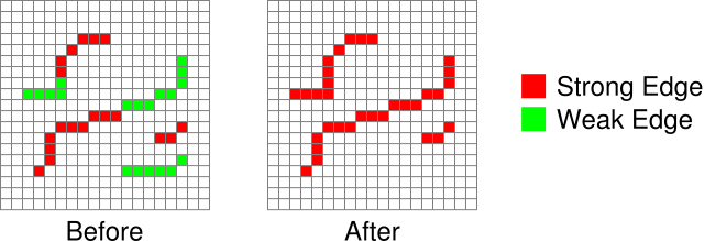
It’s finally time to finish implementing the Canny edge detector algorithm. The previous step produced an image where strong and weak edges were detected. Pixels marked as strong edges are assumed to be actual edges. On the other hand, pixels marked as weak edges are considered to only “maybe” be edges. So the question remains, when should a weak edge actually be a strong edge? If you have a chain of strong edges connected to each other, then there is definitely an edge running along them. You could then reason that if a group of weak edges are directly connected to these strong edges, they are part of the same edge and should be promoted. This is where connectivity analysis comes in.

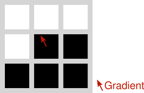
Connectivity analysis is a very mathy term but is straight forward with respect to image processing. The whole idea is about examining groups of pixels that meet some requirement and are connected in such a way that you can move from any one pixel in the group to any other without leaving the group. Say you have a pixel that meets a certain criteria. Look at each of the surrounding pixels and check if it meets a criteria (could be the same as before but doesn’t have to be). If it does, the pixels are connected. Repeat this process to find all pixels in the group. That’s it, actually really simple, right?

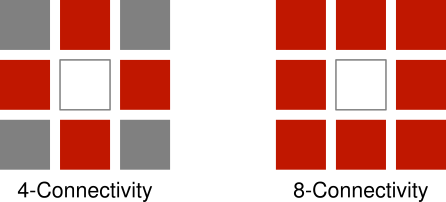
Which surrounding pixels should be examined depends on application. The two most common patterns are known as 4- and 8-connectivity. The former checks the pixels directly left, right, above, and below. The latter checks all of the same pixels as 4-connectivity but also top-left, top-right, bottom-left, and bottom-right.

In this case, we need to find strong edge pixels and then check each surrounding pixel if it’s a weak edge pixel. If it is, change it into a strong edge pixel since the strong and weak edges are connected.

You might be wondering if you can search in the reverse order. Find weak edges and check for surrounding strong edges. The answer is yes, but it’ll probably be slower because the hysteresis thresholding used to determine if an edge is strong or weak guarantees that there are at least as many weak edges as strong edges.

Code

The implementation below searches for all strong edges. Whenever a strong edge is found, a flood fill is used to examine all 8 surrounding pixels for weak edges. Found weak edges are promoted to strong edges. The flood fill repeatedly searches the 8 surrounding pixels surrounding each promoted edge until no more weak edges are found.
```
Image image; //Input: Should be output of Non-Maximum Suppression.
             //       Channel 0: Strong edge pixels.
             //       Channel 1: Weak edge pixels.
             //       Channel 2: Should be set to 0.
             //       There should be no strong edge pixels in the pixels touching the
             //       border of the image.
             //Output: Image will have all weak edges connected to strong edges changed
             //        into strong edges. Only the first channel will have useful data,
             //        the other channels should be ignored.

//Keep track of coordinates that should be searched in case they are connected.
std::stack<std::pair<unsigned int,unsigned int>> searchStack;

//Add all 8 coordinates around (x,y) to be searched.
auto PushSearchConnected = [&searchStack](const unsigned int x,const unsigned int y) {
    searchStack.push(std::make_pair(x - 1,y - 1));
    searchStack.push(std::make_pair(x    ,y - 1));
    searchStack.push(std::make_pair(x + 1,y - 1));
    searchStack.push(std::make_pair(x - 1,y));
    searchStack.push(std::make_pair(x    ,y));
    searchStack.push(std::make_pair(x + 1,y));
    searchStack.push(std::make_pair(x - 1,y + 1));
    searchStack.push(std::make_pair(x    ,y + 1));
    searchStack.push(std::make_pair(x + 1,y + 1));
};

//Find strong edge pixels and flood fill so all connected weak edges are turned into
//strong edges.
for(unsigned int y = 1;y < image.height - 1;y++)
{
    for(unsigned int x = 1;x < image.width - 1;x++)
    {
        const unsigned int index = (y * image.width + x) * 3;

        //Skip pixels that are not strong edges.
        if(image.data[index + 0] == 0)
            continue;

        //Flood fill all connected weak edges.
        PushSearchConnected(x,y);
        while(!searchStack.empty())
        {
            const std::pair<unsigned int,unsigned int> coordinates = searchStack.top();
            searchStack.pop();

            //Skip pixels that are not weak edges.
            const unsigned int x = coordinates.first;
            const unsigned int y = coordinates.second;
            const unsigned int index = (y * image.width + x) * 3;
            if(image.data[index + 1] == 0)
                continue;

            //Promote to strong edge.
            image.data[index + 0] = 255;
            image.data[index + 1] = 0;

            //Search around this coordinate as well. This will waste time checking the previous
            //coordinate again but it's fast enough.
            PushSearchConnected(x,y);
        }
    }
}
```
Putting it All Together

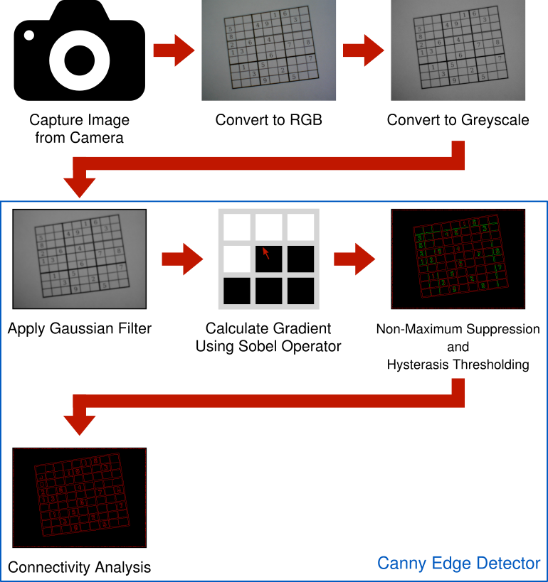
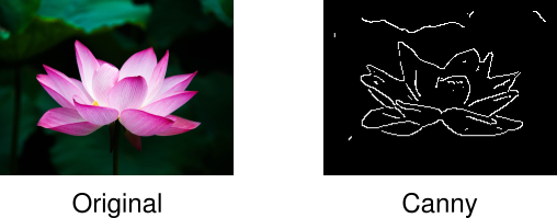
Here’s the pipeline so far. An RGB image is captured using a camera. The RGB image is converted to greyscale so it can be processed with the Canny edge detector. The Canny edge detector, applies a Gaussian filter to remove noise and suppress insignificant edges. The “flow” of the image is analyzed by finding gradients using the Sobel operator. These gradients are the measured strength and direction of change in pixel intensities. Non-Maximum Suppression is applied using the gradients to find potential edges. Hysteresis Thresholding compares the potential edge gradients strengths to a couple of thresholds which categorize if an edge is an actual edge, maybe an edge, or not an edge. Finally, Connectivity Analysis promotes those “maybe” edges to actual edges whenever they’re directly connected to an actual edge.

Besides the input image, the Canny edge detector has three tweakable parameters that can have a big impact on whether an edge is detected or not. The first is the radius of the Gaussian filter. If the radius is too large, edges are blended together and not detected. If the radius is too small, small edges or noise are detected which should be ignored. An effective radius choice is further complicated by the results depending on the size of image being used. For this project, images are 640x480 and I’ve found a radius of 5 pixels works quite well. Larger images can be downscaled which, depending on choice of sampling filter, helps to further suppress noise anyway. Smaller images are not practical because they lack a sufficient number of pixels for all of the numbered digits to be identified reliably.

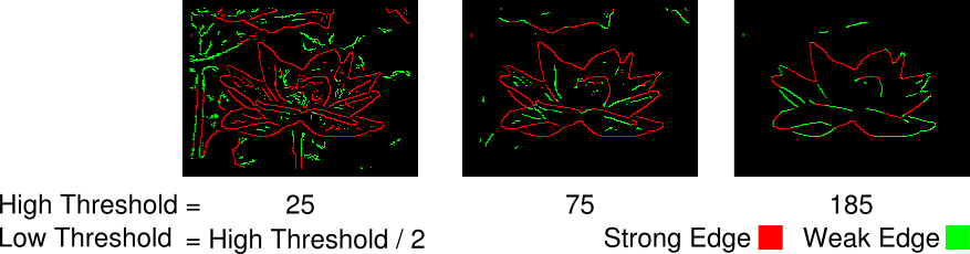
The other two parameters are the high and low thresholds used in the Hysteresis Thresholding step. These are a little trickier to get right and are problem dependent. In general, having the high threshold two or three times the low threshold works well. But that still leaves picking a high threshold. I’m using a statistical approach called Otsu’s method which is effective on high contrast images. In this case, the puzzles are usually printed in black ink on white paper which is a perfect fit. I’m not going to go over how Otsu’s method works in interest of keeping this blog series from getting any longer. However, the output hovers around 110 for all of my test cameras and puzzles so that’s probably a good place to start experimenting.

Building on the output of the Canny edge detector, the next post will cover the detection of straight lines which might indicate the grid in a Sudoku puzzle.
Sep 28, 2017
Sudoku Solver AR Part 8: Canny Part 3 (Non-Maximum Suppression)

This post is part of a series where I explain how to build an augmented reality Sudoku solver. All of the image processing and computer vision is done from scratch. See the first post for a complete list of topics.

The whole point of the Canny edge detector is to detect edges in an image. Knowing that edges are a rapid change in pixel intensity and armed with the gradient image created using the method in the previous post, locating the edges should be straight forward. Visit each pixel and mark it as an edge if the gradient magnitude is greater than some threshold value. Since the gradient measures the change in intensity and a higher magnitude means a higher rate of change, you could reason that the marked pixels are in fact edges. However, there’s a few problems with this approach. First, marked edges have an arbitrary thickness which might make it harder to determine if it’s part of a straight line. Second, noise and minor textures that were not completely suppressed by the Gaussian filter can create false positives. And third, edges which are not evenly lit (eg. partially covered by a shadow) could be partly excluded by the selected threshold.

These issues are handled using a mixture of Non-Maximum Suppression, Hysterasis Thresholding, and Connectivity Analysis. Since Non-Maximum Suppression and Hysterasis Thresholding are easily performed at the same time, I’m going to cover them together in this post. Connectivity Analysis will be covered next time as the final step in the Canny algorithm.

Non-Maximum Suppression

Non-Maximum Suppression is a line thinning technique. The basic idea isn’t all that different from the naive concept above. The magnitude of the gradient is still used to find pixels that are edges but it isn’t compared to some threshold value. Instead, it’s compared against gradients on either side of the edge, directed by the current gradient’s angle, to make sure they have smaller magnitudes.

The gradient’s angle points in the direction perpendicular to that of the edge. If you’re familiar with normals, that’s exactly what this is. Then this angle already points to one side of the edge. But both sides of the edge are compared, so rotate the angle 180 degrees to find the other side.

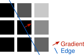
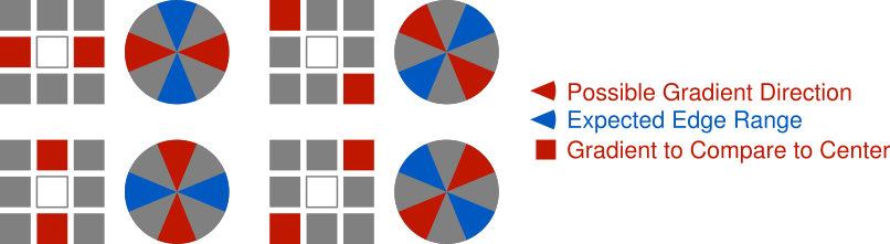
Examine one of these two angles and look at which surrounding pixels it points to. Depending on the angle, it probably won’t point directly at a single pixel. In the example above, instead of pointing directly to the right, it points a little above the right. By the discrete nature of working with images, an approximation must be used to determine a magnitude for comparison on each side of the center gradient. The angle could be snapped to point to the the nearest pixel and respective gradient or an interpolation could be performed between the gradients of the two closest matching pixels. The latter is more accurate but the former is simpler to implement and performs fine for our purpose so that’s the approach used in the code example below.

Hysterasis Thresholding

Hysterasis Thresholding is used to suppress edges that were erroneously detected by Non-Maximum Suppression. This could be noise or some pattern that’s too insignificant to be an edge. Perhaps not an obvious solution, but luckily it’s not very complicated. If the magnitude of a gradient is greater than or equal to some high threshold, mark the pixel as a strong edge. If the magnitude of a gradient is greater than or equal to some low threshold, but less than the high threshold, mark the pixel as a weak edge. A strong edge is assumed to be an actual edge where as a weak edge is “maybe” an edge. Weak edges can be promoted to strong edges if they’re directly connected to a strong edge but that’s covered in the next post. The high and low thresholds can be determined experimentally or through various statistical methods outside the scope of this post.

Code

These two concepts are easily implemented together. Start by examining each gradient’s angle to determine which surrounding gradients should be examined. If the current gradient’s magnitude is greater than both the appropriate surrounding gradients’ magnitudes, proceed to hysterasis thresholding. Otherwise, assume the pixel for the current gradient is not an edge. For the hysterasis thresholding step, mark the pixel as a strong edge if it’s greater than or equal to the specified high threshold. If not, mark the pixel as a weak edge if it’s greater than or equal to the specified low threshold. Otherwise, assume the pixel for the current gradient is not an edge. Repeat the process until every gradient is examined.

The following code marks pixels as strong or weak edges by writing to an RGB image initialized to 0. Strong edges set the red channel to 255 and weak edges set the green channel to 255. This could have easily been accomplished with a single channel image where, say, strong edges are set to 1, weak edges set to 2, and non-edges set to 0. The choice of using a full RGB image here is purely for convenience because the results are easier to examine.
```
const std::vector<float> gradient; //Input gradient with magnitude and angle interleaved
                                   //for each pixel.
const unsigned int width; //Width of image the gradient was created from.
const unsigned int height; //Height of image the gradient was created from.
const unsigned char lowThreshold; //Minimum gradient magnitude to be considered a weak
                                  //edge.
const unsigned char highThreshold; //Minimum gradient magnitude to be considered a strong
                                   //edge.
Image outputImage(width,height); //Output RGB image. A high red channel indicates a strong
                                 //edge, a high green channel indicates a weak edge, and
                                 //the blue channel is set to 0.

assert(gradient.size() == width * height * 2);
assert(lowThreshold < highThreshold);

//Perform Non-Maximum Suppression and Hysterasis Thresholding.
for(unsigned int y = 1;y < height - 1;y++)
{
    for(unsigned int x = 1;x < width - 1;x++)
    {
        const unsigned int inputIndex = (y * width + x) * 2;
        const unsigned int outputIndex = (y * width + x) * 3;

        const float magnitude = gradient[inputIndex + 0];

        //Discretize angle into one of four fixed steps to indicate which direction the
        //edge is running along: horizontal, vertical, left-to-right diagonal, or
        //right-to-left diagonal. The edge direction is 90 degrees from the gradient
        //angle.
        float angle = gradient[inputIndex + 1];

        //The input angle is in the range of [-pi,pi] but negative angles represent the
        //same edge direction as angles 180 degrees apart.
        angle = angle >= 0.0f ? angle : angle + M_PI;

        //Scale from [0,pi] to [0,4] and round to an integer representing a direction.
        //Each direction is made up of 45 degree blocks. The rounding and modulus handle
        //the situation where the first and final 45/2 degrees are both part of the same
        //direction.
        angle = angle * 4.0f / M_PI;
        const unsigned char direction = lroundf(angle) % 4;

        //Only mark pixels as edges when the gradients of the pixels immediately on either
        //side of the edge have smaller magnitudes. This keeps the edges thin.
        bool suppress = false;
        if(direction == 0) //Vertical edge.
            suppress = magnitude < gradient[inputIndex - 2] ||
                       magnitude < gradient[inputIndex + 2];
        else if(direction == 1) //Right-to-left diagonal edge.
            suppress = magnitude < gradient[inputIndex - width * 2 - 2] ||
                       magnitude < gradient[inputIndex + width * 2 + 2];
        else if(direction == 2) //Horizontal edge.
            suppress = magnitude < gradient[inputIndex - width * 2] ||
                       magnitude < gradient[inputIndex + width * 2];
        else if(direction == 3) //Left-to-right diagonal edge.
            suppress = magnitude < gradient[inputIndex - width * 2 + 2] ||
                       magnitude < gradient[inputIndex + width * 2 - 2];

        if(suppress || magnitude < lowThreshold)
        {
            outputImage.data[outputIndex + 0] = 0;
            outputImage.data[outputIndex + 1] = 0;
            outputImage.data[outputIndex + 2] = 0;
        }
        else
        {
            //Use thresholding to indicate strong and weak edges. Strong edges are assumed
            //to be valid edges. Connectivity analysis is needed to check if a weak edge
            //is connected to a strong edge. This means that the weak edge is also a valid
            //edge.
            const unsigned char strong = magnitude >= highThreshold ? 255 : 0;
            const unsigned char weak = magnitude < highThreshold ? 255 : 0;
            outputImage.data[outputIndex + 0] = strong;
            outputImage.data[outputIndex + 1] = weak;
            outputImage.data[outputIndex + 2] = 0;
        }
    }
}
```
We’re almost done implementing the Canny algorithm. Next week will be the final step where Connectivity Analysis is used to find weak edges that should be be promoted to strong edges. There will also be a quick review and some final thoughts on using the algorithm.
Sep 15, 2017
Sudoku Solver AR Part 7: Canny Part 2 (Sobel)

This post is part of a series where I explain how to build an augmented reality Sudoku solver. All of the image processing and computer vision is done from scratch. See the first post for a complete list of topics.

The second part of the Canny algorithm involves finding the gradient at each pixel in the image. This gradient is just a vector describing the relative change in intensity between pixels. Since a vector has a magnitude and a direction, then this gradient describes how much the intensity is changing and in what direction.

The gradient is found using the Sobel operator. The Sobel operator uses two convolutions to measure the rate of change in intensity using surrounding pixels. If you studied Calculus, it’s worth noting that this is just a form of differentiation. One convolution measures the horizontal direction and the other measures the vertical direction. These two values together form the gradient vector. Below are the most common Sobel kernels. Unlike the Gaussian kernel, the Sobel kernels do not change so they can simply be hard coded.

`K_x = [[-1,0,1],[-2,0,2],[-1,0,1]]`

`K_y = [[-1,-2,-1],[0,0,0],[1,2,1]]`

Where `K_x` is the horizontal kernel and `K_y` is the vertical kernel.

A little more processing is needed to make the gradient usable for the Canny algorithm. If you’ve studied linear algebra or are familiar with polar coordinates the following should be familiar to you.

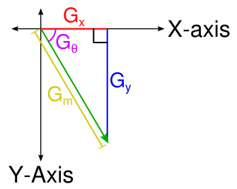
First, the magnitude is needed which describes how quickly the intensity of the pixels are changing. By noting that the result of each convolution describes a change along the x- and y-axis, these two pairs put together form the adjacent and opposite sides of a right triangle. From there it should follow immediately that the magnitude is the length of the hypotenuse and can be solved using Pythagorean theorem.

`G_m = sqrt(G_x^2 + G_y^2)`

Where `G_m` is the magnitude, `G_x` is the result of the horizontal convolution, and `G_y` is the result of the vertical convolution.

The direction of the gradient in radians is also needed. Using a little trigonometry and the fact that we can calculate the tangent using the `G_x` and `G_y` components

`tan(G_theta) = G_y / G_x`

`G_theta = arctan(G_y / G_x)`

Where `G_theta` is the angle in radians. The `arctan` term requires special handling to prevent a divide by zero. Luckily, C++ (and most programming languages) have a convenient atan2 function that handles this case by conveniently returning `+-0` or `+-pi`. The C++ variant of atan2 produces radians in the range `[-pi,pi]` with `0` pointing down the positive x-axis and the angle proceeding in a clockwise direction.

The following example demonstrates how to calculate the gradient for a region of pixels. A typical unsigned 8-bit data type is assumed with the black pixels having a value of 0 and the white pixels having a value of 255.

`P = [[255,255,255],[255,0,0],[0,0,0]]`

`G_x = P ** K_x = (255 * -1) + (255 * 0) + (255 * 1) + (255 * -2) + (0 * 0) + (0 * 2) + (0 * -1) + (0 * 0) + (0 * 1) = -510`

`G_y = P ** K_y = (255 * -1) + (255 * -2) + (255 * -1) + (255 * 0) + (0 * 0) + (0 * 0) + (0 * 1) + (0 * 2) + (0 * 1) = -1020`

`G_m = sqrt((-510)^2 + (-1020)^2) = 1140.39467`

`G_theta = arctan((-1020)/-510) = -2.03444 text{ radians} = 4.24888 text{ radians}`

Here’s an implementation in code that, once again, ignores the border where the convolution would access out of bounds pixels.
```
const Image image; //Input RGB greyscale image
                   //(Red, green, and blue channels are assumed identical).
std::vector<float> gradient(image.width * image.height * 2,0.0f); //Output gradient with
                                                                  //magnitude and angle
                                                                  //interleaved.

//Images smaller than the Sobel kernel are not supported.
if(image.width < 3 || image.height < 3)
    return;

//Number of items that make up a row of pixels.
const unsigned int rowSpan = image.width * 3;

//Calculate the gradient using the Sobel operator for each non-border pixel.
for(unsigned int y = 1;y < image.height - 1;y++)
{
    for(unsigned int x = 1;x < image.width - 1;x++)
    {
        const unsigned int inputIndex = (y * image.width + x) * 3;

        //Apply the horizontal Sobel kernel.
        const float gx =
            static_cast<float>(image.data[inputIndex - rowSpan - 3]) * -1.0f + //Top left
            static_cast<float>(image.data[inputIndex - rowSpan + 3]) *  1.0f + //Top right
            static_cast<float>(image.data[inputIndex - 3])           * -2.0f + //Mid left
            static_cast<float>(image.data[inputIndex + 3])           *  2.0f + //Mid right
            static_cast<float>(image.data[inputIndex + rowSpan - 3]) * -1.0f + //Bot left
            static_cast<float>(image.data[inputIndex + rowSpan + 3]) *  1.0f;  //Bot right

        //Apply the vertical Sobel kernel.
        const float gy =
            static_cast<float>(image.data[inputIndex - rowSpan - 3]) * -1.0f + //Top left
            static_cast<float>(image.data[inputIndex - rowSpan])     * -2.0f + //Top mid
            static_cast<float>(image.data[inputIndex - rowSpan + 3]) * -1.0f + //Top right
            static_cast<float>(image.data[inputIndex + rowSpan - 3]) *  1.0f + //Bot left
            static_cast<float>(image.data[inputIndex + rowSpan])     *  2.0f + //Bot mid
            static_cast<float>(image.data[inputIndex + rowSpan + 3]) *  1.0f;  //Bot right

        //Convert gradient from Cartesian to polar coordinates.
        const float magnitude = hypotf(gx,gy); //Computes sqrt(gx*gx + gy*gy).
        const float angle = atan2f(gy,gx);

        const unsigned int outputIndex = (y * image.width + x) * 2;
        gradient[outputIndex + 0] = magnitude;
        gradient[outputIndex + 1] = angle;
    }
}
```
Next is another step in the Canny algorithm which uses the gradient created here to build an image with lines where edges were detected in the original image.
Aug 31, 2017
Sudoku Solver AR Part 6: Canny Part 1 (Gaussian Blur)

This post is part of a series where I explain how to build an augmented reality Sudoku solver. All of the image processing and computer vision is done from scratch. See the first post for a complete list of topics.

We captured an image from a connected camera (Linux, Windows) and converted it to greyscale. Now to start searching for a puzzle in the image. Since puzzles are made up of a grid of lines, it makes sense that the goal should be to hunt down these straight lines. But how should this be done exactly? It sure would be nice if an image could have all of its shading removed and be left with just a bunch of outlines. Then maybe it would be easier to find straight lines. Enter, the Canny edge detector.

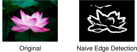
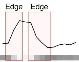
Take a row of pixels from a typical greyscale image and line graph them by intensity. Some sections of the graph will change very little. Other parts will have a much more rapid change indicating an edge in the image. The Canny edge detector is a multi-step algorithm used to find such edges in an image. A particularly nice property of the algorithm is edges are usually reduced to a thickness of a single pixel. It’s very useful considering the thickness of an edge can vary as you move along it.

Gaussian Blur

The first step is to apply a Gaussian filter to the image. Gaussian filters are used for blurring images. They’re very good for suppressing insignificant detail such as the noise introduced by a camera’s capture process.

The Gaussian filter is a convolution based on the Gaussian function (very commonly used in statistics where it describes the normal distribution). Plotting the function produces a bell shaped curve. It’s usually described using the following formula:

`text{Gaussian}(x) = 1/(sigma^2 sqrt(2pi)) * e^(-x^2/(2sigma^2))`

Where x is the distance from the center of the curve and `sigma` is the standard deviation. The standard deviation is used to adjust the width of the bell curve. The constant multiplier at the beginning is used as a normalizing term so the area under the curve is equal to 1. Since we’re only interested in a discrete form of the function that’s going to require normalization (more on this in a moment) anyway, this part can be dropped.

`text{Gaussian}(x) = e^(-x^2/(2sigma^2))`

The standard deviation choice is somewhat arbitrary. A larger standard deviation indicates data points spread out further relative from the mean have more significance. In this case, the mean is the center of the filter where `x = 0` and significance is the contribution to the output pixel. A convenient method is to choose a factor representing how many standard deviations from the mean should be considered significant and relating it to the radius of the filter in pixels.

`r = a*sigma`

`sigma = r/a`

Where `r` is the radius, `sigma` is the standard deviation, and `a` is the number of standard deviations. In the case of image processing, letting `a = 3` is usually sufficient.

`r`:

`a`:

A convenient property of the Gaussian filter is it’s a separable filter which means that instead of building a 2D (square) convolution matrix, only a 1D convolution matrix is necessary. Then the convolution is applied in one horizontal pass and one separate vertical pass. Not only does this run faster in practice, but it also simplifies the code.

The first step is to build a kernel by sampling the Gaussian function, defined above, at discrete steps. Then the kernel must be normalized so the sum of each of its values is 1. Normalization is performed by summing all of the values in the kernel and dividing each value by this sum. If the kernel is not normalized, using it in a convolution will make the resulting image either darker or lighter depending on if the sum of the kernel is less than or greater than 1, respectively.
```
const float radius; //Radius of kernel in pixels. Can be decimal.
const float sigma = radius / 3.0f; //Sigma chosen somewhat arbitrarily.
const unsigned int kernelRadius = static_cast<unsigned int>(radius) + 1; //Actual discrete
                                                                         //sample radius.
                                                                         //The + 1 helps
                                                                         //to account for
                                                                         //the decimal
                                                                         //portion of the
                                                                         //specified
                                                                         //radius.
const unsigned int kernelSize = kernelRadius * 2 + 1; //Number of values in the kernel.
                                                      //Includes left-side, right-side,
                                                      //and center pixel.
std::vector<float> kernel(kernelSize,0.0f); //Final kernel values.

//Having a radius of 0 is equivalent to performing no blur.
if(radius == 0.0f)
    return;

//Compute the Gaussian. Straight from the formula given above.
auto Gaussian = [](const float x,const float sigma) {
    const float x2 = x * x;
    const float sigma2 = sigma * sigma;
    return expf(-x2/(2.0f*sigma2));
};

//Sample Gaussian function in discrete increments. Technically the function is symmetric
//so only the first `kernelRadius + 1` values need to be computed and the rest can be
//found by copying from the first half. But that's more complicated to implement and
//isn't worth the effort.
float sum = 0.0f; //Keep an accumulated sum for normalization.
for(unsigned int x = 0;x < kernelSize;x++)
{
    const float value = Gaussian(static_cast<float>(x) -
                                 static_cast<float>(kernelRadius),sigma);
    kernel[x] = value;

    sum += value;
}

//Normalize kernel values so they sum to 1.
for(float& value : kernel)
{
    value /= sum;
}
```
Applying the kernel is done by performing a convolution in separate horizontal and vertical passes. I’m choosing to ignore the edges here because they aren’t necessary for this project. If you need them, clamping to the nearest non-out-of-bounds pixels works well.
```
const std::vector<float> kernel; //Gaussian kernel computed above.
const unsigned int kernelRadius; //Gaussian kernel radius computed above.
const Image inputImage; //Input RGB image.
Image outputImage(inputImage.width,inputImage.height); //Output RGB image. Same width and
                                                       //height as inputImage. Initialized
                                                       //so every pixel is set to (0,0,0).

assert(kernel.size() == kernelRadius * 2 + 1);

//Convenience function for clamping a float to an unsigned 8-bit integer.
auto ClampToU8 = [](const float value)
{
    return static_cast<unsigned char>(std::min(std::max(value,0.0f),255.0f));
};

//Since the input image is not blurred around the border in this implementation, then the
//output would just be a blank image if the image is smaller than this area.
if(kernelRadius * 2 > inputImage.width || kernelRadius * 2 > inputImage.height)
    return outputImage;

//Blur horizontally. Save the output to a temporary buffer because the convolution can't
//be performed in place. This also means the output of the vertical pass can be placed
//directly into the output image.
std::vector<unsigned char> tempImageData(inputImage.data.size()); //Temporary RGB image
                                                                  //data used between
                                                                  //passes.
for(unsigned int y = 0;y < inputImage.height;y++)
{
    for(unsigned int x = kernelRadius;x < inputImage.width - kernelRadius;x++)
    {
        float sum[3] = {0.0f,0.0f,0.0f};
        for(unsigned int w = 0;w < kernel.size();w++)
        {
            const unsigned int inputIndex =
                (y * inputImage.width + x + w - kernelRadius) * 3;
            sum[0] += static_cast<float>(inputImage.data[inputIndex + 0]) * kernel[w];
            sum[1] += static_cast<float>(inputImage.data[inputIndex + 1]) * kernel[w];
            sum[2] += static_cast<float>(inputImage.data[inputIndex + 2]) * kernel[w];
        }

        const unsigned int outputIndex = (y * inputImage.width + x) * 3;
        tempImageData[outputIndex + 0] = ClampToU8(sum[0]);
        tempImageData[outputIndex + 1] = ClampToU8(sum[1]);
        tempImageData[outputIndex + 2] = ClampToU8(sum[2]);
    }
}

//Blur vertically. Notice that the inputIndex for the weights is incremented across the
//y-axis instead of the x-axis.
for(unsigned int y = kernelRadius;y < inputImage.height - kernelRadius;y++)
{
    for(unsigned int x = kernelRadius;x < inputImage.width - kernelRadius;x++)
    {
        float sum[3] = {0.0f,0.0f,0.0f};
        for(unsigned int w = 0;w < kernel.size();w++)
        {
            const unsigned int inputIndex =
                ((y + w - kernelRadius) * inputImage.width + x) * 3;
            sum[0] += static_cast<float>(tempImageData[inputIndex + 0]) * kernel[w];
            sum[1] += static_cast<float>(tempImageData[inputIndex + 1]) * kernel[w];
            sum[2] += static_cast<float>(tempImageData[inputIndex + 2]) * kernel[w];
        }

        const unsigned int outputIndex = (y * inputImage.width + x) * 3;
        outputImage.data[outputIndex + 0] = ClampToU8(sum[0]);
        outputImage.data[outputIndex + 1] = ClampToU8(sum[1]);
        outputImage.data[outputIndex + 2] = ClampToU8(sum[2]);
    }
}
```
While the Canny edge detector described here going forward expects a greyscale image, the Gaussian filter works well on RGB or most other image formats. Next time I’ll cover the next step of the Canny edge detector which involves analyzing how the intensity and direction of pixels change throughout an image.

Aug 17, 2017

Sudoku Solver AR Part 5: Camera Capture (Windows)

This post is part of a series where I explain how to build an augmented reality Sudoku solver. All of the image processing and computer vision is done from scratch. See the first post for a complete list of topics.

Video frames from a camera are captured on Windows (Vista and later) using the Media Foundation API. The API is designed to handle video/audio capture, processing, and rendering. And… it’s really a pain to work with. The documentation contains so many words, yet requires jumping all over the place and never seems to explain what you want to know. Adding insult to injury, Media Foundation is a COM based API, so you can expect lots of annoying reference counting.

Hopefully, I scared you into using a library for your own projects. Otherwise, just like with the Linux version of this post, I’m going to go over how to find all of the connected cameras, query their supported formats, capture video frames, and convert them to RGB images.

List Connected Cameras

A list of connected cameras can be found using the MFEnumDeviceSources function. A pointer to an IMFAttributes must be provided to specify the type of devices that should be returned. To find a list of cameras, video devices should be specified. IMFAttributes is basically a key-value store used by Media Foundation. A new instance can be created by calling the MFCreateAttributes function.

After evaluating the available video devices, make sure to clean-up the unused devices by calling Release on each and CoTaskMemFree on the array of devices. This behavior of having to manually manage referencing counting everywhere within Media Foundation. It makes proper error handling incredibly tedious so I’ve only inserted assert() calls in the following code snippets for brevity.

#include <mfapi.h>

...

//Create an instance of IMFAttributes. This class is basically a key-value store used by
//many Media Foundation functions to configure how they should behave.
IMFAttributes* attributes = nullptr;
HRESULT hr = MFCreateAttributes(&attributes,1);
assert(SUCCEEDED(hr));

//Configure the MFEnumDeviceSources call below to look for video capture devices only.
hr = attributes->SetGUID(MF_DEVSOURCE_ATTRIBUTE_SOURCE_TYPE,
                         MF_DEVSOURCE_ATTRIBUTE_SOURCE_TYPE_VIDCAP_GUID);
assert(SUCCEEDED(hr));

//Enumerate all of the connected video capture devices. Other devices besides cameras
//might be found like video capture cards.
UINT32 deviceCount = 0;
IMFActivate** devices = nullptr;
hr = MFEnumDeviceSources(attributes,&devices,&deviceCount);
assert(SUCCEEDED(hr));

//Evaluate which video devices should be used. The others should be freed by calling
//Release().
for(UINT32 x = 0;x < deviceCount;x++)
{
    IMFActivate* device = devices[x];

    //Use/store device here OR call Release() to free.

    device->Release();
}

//Clean up attributes and array of devices. Note that the devices themselves have not been
//cleaned up unless Release() is called on each one.
attributes->Release();
CoTaskMemFree(devices);

Using a Camera

Before anything can be done with a camera, an IMFMediaSource must be fetched from the device. It’s used for starting, pausing, or stopping capture on the device. None of which is necessary for this project since the device is expected to be always running. But, the IMFMediaSource is also used for creating an IMFSourceReader which is required for querying supported formats or making use of captured video frames.

#include <mfidl.h>
#include <mfreadwrite.h>

...

IMFActivate* device; //Device selected above.

//Get a media source for the device to access the video stream.
IMFMediaSource* mediaSource = nullptr;
hr = device->ActivateObject(__uuidof(IMFMediaSource),
                            reinterpret_cast<void**>(&mediaSource));
assert(SUCCEEDED(hr));

//Create a source reader to actually read from the video stream. It's also used for
//finding out what formats the device supports delivering the video as.
IMFSourceReader* sourceReader = nullptr;
hr = MFCreateSourceReaderFromMediaSource(mediaSource,nullptr,&sourceReader);
assert(SUCCEEDED(hr));

...

//Clean-up much later when done querying the device or capturing video.
mediaSource->Release();
sourceReader->Release();

Querying Supported Formats

Cameras capture video frames in different sizes, pixel formats, and rates. You can query a camera’s supported formats to find the best fit for your use or just let the driver pick a sane default.

There’s certainly an advantage to picking the formats yourself. For example, since cameras rarely provide an RGB image, if a camera uses a format that you already know how to convert to RGB, you can save time and use that instead. You can also choose to lower the frame rate for better quality at a cost of more motion blur or raise the frame rate for a more noisy image and less motion blur.

The supported formats are found by repeatedly calling the GetNativeMediaType method on the IMFSourceReader instance created above. After each call, the second parameter is incremented until the function returns an error indicating that there are no more supported formats. The actual format info is returned in the third parameter as an IMFMediaType instance. IMFMediaType inherits from the IMFAttributes class used earlier so it also behaves as a key-value store. The keys used to look up info about the current format are found on this page.

IMFSourceReader* sourceReader; //Source reader created above.

//Iterate over formats directly supported by the video device.
IMFMediaType* mediaType = nullptr;
for(DWORD x = 0;
    sourceReader->GetNativeMediaType(MF_SOURCE_READER_FIRST_VIDEO_STREAM,
                                     x,
                                     &mediaType) == S_OK;
    x++)
{
    //Query video pixel format. The list of possible video formats can be found at:
    //https://msdn.microsoft.com/en-us/library/windows/desktop/aa370819(v=vs.85).aspx
    GUID pixelFormat;
    hr = mediaType->GetGUID(MF_MT_SUBTYPE,&pixelFormat);
    assert(SUCCEEDED(hr));

    //Query video frame dimensions.
    UINT32 frameWidth = 0;
    UINT32 frameHeight = 0;
    hr = MFGetAttributeSize(mediaType,MF_MT_FRAME_SIZE,&frameWidth,&frameHeight);
    assert(SUCCEEDED(hr));

    //Query video frame rate.
    UINT32 frameRateNumerator = 0;
    UINT32 frameRateDenominator = 0;
    hr = MFGetAttributeRatio(mediaType,
                             MF_MT_FRAME_RATE,
                             &frameRateNumerator,
                             &frameRateDenominator);
    assert(SUCCEEDED(hr));

    //Make use of format, size, and frame rate here or hold onto mediaType as is (don't
    //call Release() next) for configuring the camera (see below).

    //Clean-up mediaType when done with it.
    mediaType->Release();
}

Selecting a Format

There’s not a lot to setting the device to use a particular format. Just call the SetCurrentMediaType method on the IMFSourceReader instance and pass along one of the IMFMediaType queried above.

IMFSourceReader* sourceReader; //Source reader created above.
IMFMediaType* mediaType; //Media type selected above.

//Set source reader to use the format selected from the list of supported formats above.
hr = sourceReader->SetCurrentMediaType(MF_SOURCE_READER_FIRST_VIDEO_STREAM,
                                       nullptr,
                                       mediaType);
assert(SUCCEEDED(hr));

//Clean-up mediaType since it won't be used anymore.
mediaType->Release();

Capturing a Video Frame

There’s a couple of ways to capture a video frame using Media Foundation. The method described here is the synchronous approach which is the simpler of the two. Basically, the process involves asking for a frame of video whenever we want a one and the thread then blocks until a new frame is available. If frames are not requested fast enough, they get dropped and a gap is indicated.

This is done by calling the ReadSample method on the IMFSourceReader instance. This function returns an IMFSample instance or a nullptr if a gap occurred. The IMFSample is a container that stores various information about a frame including the actual data in the pixel format selected above.

Accessing the pixel data involves calling the GetBufferByIndex method of the IMFSample and calling Lock on the resulting IMFMediaBuffer instance. Locking the buffer prevents the frame data from being modified while you’re processing it. For example, the operating system might want to re-use the buffer for frames in the future but writing to it at the same tile as it’s being read will garble the image.

Once done working with the frame data, don’t forget to call Unlock on it and clean-up IMFSample and IMFMediaBuffer in preparation for future frames.

IMFSourceReader* sourceReader; //Source reader created above.

//Grab the next frame. A loop is used because ReadSample returns a null sample when there
//is a gap in the stream.
IMFSample* sample = nullptr;
while(sample == nullptr)
{
    DWORD streamFlags = 0; //Most be passed to ReadSample or it'll fail.
    hr = sourceReader->ReadSample(MF_SOURCE_READER_FIRST_VIDEO_STREAM,
                                  0,
                                  nullptr,
                                  &streamFlags,
                                  nullptr,
                                  &sample);
    assert(SUCCEEDED(hr));
}

//Get access to the underlying memory for the frame.
IMFMediaBuffer* buffer = nullptr;
hr = sample->GetBufferByIndex(0,&buffer);
assert(SUCCEEDED(hr));

//Begin using the frame's data.
BYTE* bufferData = nullptr;
DWORD bufferDataLength = 0;
hr = buffer->Lock(&bufferData,nullptr,&bufferDataLength);
assert(SUCCEEDED(hr));

//Copy buffer data or convert directly to RGB here. The frame format, width, and height
//match the media type set above.

//Stop using the frame's data.
buffer->Unlock();

//Clean-up sample and buffer since frame is no longer being used.
sample->Release();
buffer->Release();

Converting a Video Frame To RGB

The selected pixel format probably cannot be used directly. For our use, it needs to be converted to RGB¹. The conversion process varies by format. In the last post I covered the YUYV 4:2:2 format. In this one, I’m going to go over the similar NV12 format.

The NV12 format is a Y’CbCr format that’s split into two chunks. The first chunk is the luminance (Y’) channel which contains an entry for each pixel. The second chunk interleaves the Cb and Cr channels together. There are only one Cb and Cr pair for every 2x2 region of pixels.

Just like with the YUYV 4:2:2 format, the Y’CbCr to RGB conversion can be done by following the JPEG standard. This is a sufficient approach because we are assuming the camera’s color space information is unavailable.

`R = Y’ + 1.402 * (Cr - 128)`

`G = Y’ - 0.344 * (Cb - 128) - 0.714 * (Cr - 128)`

`B = Y’ + 1.772 * (Cb - 128)`

const unsigned int imageWidth; //Width of image.
const unsigned int imageHeight; //Height of image.
const std::vector<unsigned char> nv12Data; //Input NV12 buffer read from camera.
std::vector<unsigned char> rgbData(imageWidth * imageHeight * 3); //Output RGB buffer.

//Convenience function for clamping a signed 32-bit integer to an unsigned 8-bit integer.
auto ClampToU8 = [](const int value)
{
    return std::min(std::max(value,0),255);
};

const unsigned int widthHalf = imageWidth / 2;

//Convert from NV12 to RGB.
for(unsigned int y = 0;y < imageHeight;y++)
{
    for(unsigned int x = 0;x < imageWidth;x++)
    {
        //Clear the lowest bit for both the x and y coordinates so they are always even.
        const unsigned int xEven = x & 0xFFFFFFFE;
        const unsigned int yEven = y & 0xFFFFFFFE;

        //The Y chunk is at the beginning of the frame and easily indexed.
        const unsigned int yIndex = y * imageWidth + x;

        //The Cb and Cr channels are interleaved in their own chunk after the Y chunk.
        //This chunk is 1/4th the size of the first chunk. There is one Cb and one Cr
        //component for every 2x2 region of pixels.
        const unsigned int cIndex = imageWidth * imageHeight + yEven * widthHalf + xEven;

        //Extract YCbCr components.
        const unsigned char y = nv12Data[yIndex];
        const unsigned char cb = nv12Data[cIndex + 0];
        const unsigned char cr = nv12Data[cIndex + 1];

        //Convert from YCbCr to RGB.
        const unsigned int outputIndex = (y * imageWidth + x) * 3;
        rgbData[outputIndex + 0] = ClampToU8(y + 1.402 * (cr - 128));
        rgbData[outputIndex + 1] = ClampToU8(y - 0.344 * (cb - 128) - 0.714 * (cr - 128));
        rgbData[outputIndex + 2] = ClampToU8(y + 1.772 * (cb - 128));
    }
}

That’s it for video capture, now the image is ready to be processed. I’m going to repeat what I said in the opening, go find a library to handle all of this for you. Save yourself the hassle. Especially if you decide to support more pixel formats or platforms in the future. Next up will be the Canny edge detector which is used to find edges in an image.

Footnotes

I have a camera that claims to produce RGB images but actually gives BGR (red and blue are switched) images with the rows in bottom-to-top order. Due to the age of the camera, the hardware is probably using the .bmp format which is then directly unpacked by the driver. Anyway, expect some type of conversion to always be necessary. ↩

1 2 Next

`r`:
`a`:

Posts

Sudoku Solver AR Part 9: Canny Part 4 (Connectivity Analysis)

Code

Putting it All Together

Sudoku Solver AR Part 8: Canny Part 3 (Non-Maximum Suppression)

Non-Maximum Suppression

Hysterasis Thresholding